RAKK 2019: NON-DESTRUCTIVE MATERIAL TESTING WITH ACTIVE THERMOGRAPHY

Eric Rahne, B.Sc. in Electrical Engineering, forensic expert, Level 3 accredited thermography expert (Termograph Level3) (PIM Ltd.)

SUMMARY Thermography is one of the most versatile and widespread testing methods. Within this field, active thermography is increasingly used, allowing for non-destructive material testing. In active thermography, energy is deliberately applied to the object to obtain measurement results. Its capabilities lie in the mathematical evaluation of measurements, thanks to increased thermal resolution and independence from the emissivity factor. 1. INTRODUCTION Thermography has become one of the most versatile and widespread testing methods - not only in industry but also in research and development. Most applications fall under passive thermography. Active thermography is becoming more common, offering possibilities for non-destructive material testing. Active thermography includes thermal measurements/procedures where energy is deliberately applied to the object to obtain measurement results. It doesn't matter how this energy transfer is done, whether through electromagnetic waves (light or heat radiation), convection, or mechanical means (e.g., ultrasound). The potential of active thermography lies in the mathematical processing of measurement results. By applying mathematics, temperature differences even an order of magnitude smaller than what the thermal camera's capabilities (NETD value) allow can be detected. Moreover, all (presented in the presentation) mathematical evaluation procedures are independent of the object surface's emissivity factor. This provides invaluable advantages, especially in the presence of surfaces with different emissivity factors. 2. ACTIVE THERMOGRAPHY METHODS2.1. Transmission Method (thermal) Good results can be expected when using this method for thin, good thermal conductive materials. Since the energy input occurs from the back of the object, and the resulting temperature changes due to energy input are recorded on the front, any inhomogeneities in the material causing differences in thermal conductivity lead to different temperatures on the observation side. Differences can be expected not only in peak temperatures but also in the appearance time of the temperature response.

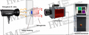
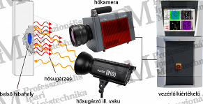
2.2. Illumination Method (heat dissipation) In these methods, energy input occurs from the observation side. It is recommended when detecting surface-near defects in weakly thermally conductive or particularly thick materials. Depending on the method, we either sense surface temperatures or temperature changes due to energy input based on emitted radiation or focus on detecting reflected radiation on the surface.

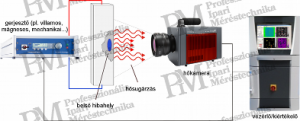
2.3. "Internally excited" thermal effect measurement Since we introduce energy into the object's interior, the measurement setup, depending on the energy source required to generate the necessary thermal effect, can be compared to the transmission method setup. Excitation can be any electrical or mechanical process capable of generating heat inside the object. Depending on the physical characteristics of the defect, the temperature measurable near the defect may be either lower or higher.

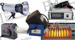
3. ENERGY INPUT OPTIONS To induce the necessary temperature changes for active thermography, the right amount of energy must be applied to the object at the right time. Various tools are commonly used depending on the properties of the object being measured and the required energy quantity. Energy input can be external or internal excitation. External excitation can be radiation (heat or light) or convection, while internal excitation can be direct electrical, inductive, or mechanical. The primary consideration in selecting the most suitable energy source is to achieve the required energy level for active thermographic observations with minimal but targeted energy input.

4. THEORY OF ACTIVE THERMOGRAPHY Let's start with the question: what makes active thermography different from passive thermography? Passive thermography often starts from steady-state, static, or quasi-steady-state thermal conditions, as seen in building insulation surveys, for example. During measurements, we utilize the object's own temperature, heat generation, or heat capacity. However, many thermal processes can be considered more dynamic than static. Compared to mechanical or electrical phenomena, they have at most a very long time constant. How long exactly? For example, the earth layer above a good wine cellar is so thick that the summer heat reaches the vault only in the cold winter. Since discussing the complete theoretical background in a twenty-minute presentation is impossible, we will focus on the two most common excitation modes and their mathematical evaluation in the following. 4.1. Excitation with temperature sinusoidal wave In the case of sinusoidal temperature variation excitation on the object, the heat conduction equation provides an extremely damped temperature wave that propagates along the distance and varies over time. The heat wave propagation equation for sinusoidal excitation is: 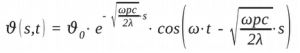formula (1) Legend: ϑ ... temperature (time- and location-dependent) [°C] c ... specific heat [J/kg ·K] ρ ...Specific gravity [kg/m3] λ ... thermal conductivity [W/m ·K] s ... temperature wave depth [m] ω ... energy input circular frequency

Assuming sinusoidal excitation, the equation for the thermal penetration depth (µ) is: 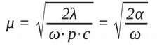formula (2) Since the damping (second multiplier) in equation (1) is far greater than the factor indicating the waveform itself, the temperature wave smears out / disappears in space and time. Using mathematical terminology, the phenomenon is aperiodic. Based on the above, the maximum depth significantly influenced by temperature excitation can be interpreted. In a material depth of one unit of µ (penetration depth) (s), only one-third (precisely: 37%) of the excitation temperature is generated. Taking the 10% value of the surface temperature as a threshold, we obtain the practical "threshold value" of the thermal penetration depth (µ10%): 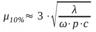formula (3) 4.2. Excitation with Temperature Impulse If we choose a temperature impulse signal-shaped excitation instead of sinusoidal temperature fluctuations, the mathematical model of the temperature wave for sinusoidal excitation is modified as follows:

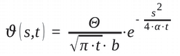
formula (4) Explanation of symbols: ϑ ... temperature (time- and location-dependent) [°C] Θ ... energy input [J] b ... heat absorption material characteristic [W√s/(m2 ·K)] α ... temperature propagation factor [m2/s] s ... temperature wave depth [m] t ... time elapsed since impulse [s] Since in this case also the damping far exceeds the value of the temperature wave, similar to sinusoidal excitation, the maximum penetration depth can be estimated. Using the assumed 10% surface temperature threshold, we now get the following estimate: formula (5) The following figure provides an explanation regarding penetration.

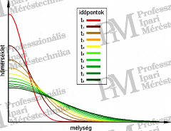
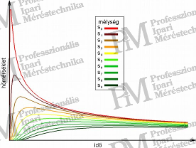
It can be recognized from the previous figures that the peak temperature occurs at a certain depth only after a (material property-dependent) time. The time can be calculated with the following equation: 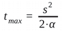formula (6) Explanation of symbols: α ... temperature propagation factor [m2/s] s ... temperature wave depth [m] t ... time elapsed since impulse [s]

5. MATHEMATICAL EVALUATION The mathematical processing and evaluation of active thermography measurement results can be done in various ways. The simplest method is to evaluate absolute temperature values without any mathematical analysis. However, this is neither efficient nor does it exploit the possibilities inherent in active thermography. Instead, the following three methods are commonly used: 5.1. Ratio-based Approach This method is mathematically the simplest. We only need to capture two thermal images: one at the beginning of the heating process and one at the end. In order to minimize the influence of environmental temperatures and the uneven temperature distribution of the initial state on our measurement results, it is advisable to capture the two values after the first 1/10 and then 9/10 of the total process time. The two values are then simply divided. Since the emissivity value of the object surface is the same for both data, we obtain emissivity-independent results!

The calculation method is incredibly simple: 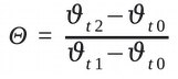formula (7) 5.2. Impulse Excitation Thermography The response of an object to a single heat impulse excitation can be examined by discrete Fourier transformation for different frequencies of amplitude and phase. For this, N thermal images need to be captured, which can be analyzed for the n-th (max. N/2 [Hz]) frequency according to the following mathematical steps. Discrete Fourier transformation for the n-th frequency (per pixel!): 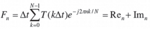formula (8) Explanation of symbols: Fn ... n-th frequency [Hz] N ... number of recorded time samples ∆t ... sampling interval T .... temperature Ren ... real value at n-th frequency Imn ... imaginary value at n-th frequency The pixels of the amplitude thermal image for the n-th frequency: 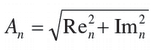formula (9) The pixels of the phase image for the n-th frequency: 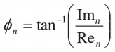formula (10) Based on the calculated pixel data, they can be visualized again using the customary color scales in thermography. Often, the phase image better represents the inhomogeneities of materials. 5.3. Sinusoidal (Lock-In) Excitation Thermography In the case of sinusoidal excitation, it is obvious that the temperature response to this periodic excitation is analyzed for amplitude and phase components using Fourier transformation.

If the reference signal is a harmonic signal (e.g. sinusoidal), then we can talk about two-channel correlation. In this case, both the amplitude and phase angle correlation can be calculated. The equation: formula (11) Explanation of symbols: ϑmeasured ... measured temperature amplitude [°C] fref ... excitation frequency [Hz] φ ... phase angle Due to the discrete sampling of data by thermal cameras, the above equation is replaced by the discrete Fourier transformation, based on which the following correlation relationship can be expressed: 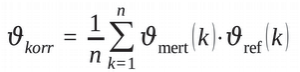formula (12) Explanation of symbols: ϑcorr ... cross-correlation temperature value [°C] ϑmeasured(k) ... k-th sampled measured temperature [°C] ϑref(k) ... k-th sampled excitation temperature [°C] n ... number of recorded samples If k → ∞ is valid, and the sampling of the signal sequence is synchronized precisely with the frequency and phase angle of the reference signal, then with a sufficient number of samples, not only the match with the excitation can be determined, but also a useful signal can be filtered out from a very noisy signal. The equation for noise filtering: 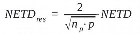formula (13) where: np = {1/a or a, a = positive integer} p = positive integer Explanation of symbols: np ... number of samples per period p ... number of periods

6. APPLICATION EXAMPLES6.1. Examination of layered plastic structures Non-destructive testing of the quality, integrity, and homogeneity of layered or fiber-reinforced plastics is becoming increasingly important in the aerospace and automotive industries. Traditional ultrasound or X-ray inspections may not provide sufficiently accurate answers for everything, and their applicability is limited. Active thermography offers new possibilities.

left: "usual" thermal image pulsed phase thermography right: ratio formation sinusoidal phase thermography 6.2. Inspection of aircraft wing flaps In terms of measurement equipment requirements and mathematical evaluation, the application of active thermography is simplest for inspecting the wing flaps of large passenger aircraft.

6.3. Inspection and qualification of welds Whether it is traditional spot welding or laser welding, by introducing short energy input at the welding location for inspection, the increasing temperature appearing on the opposite side practically outlines the location of the weld and the shape of the melted metal surface.

6.4. Inspection and qualification of riveting The following example demonstrates the application of ultrasonic-excited active thermography in aircraft maintenance.

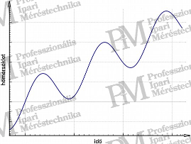
6.5. Measurement of fast periodic processes If a thermal process needs to be recorded that is periodic in nature but has a frequency that exceeds the capabilities of the thermographic system for image refresh, active thermography can still be helpful. It is only necessary to take advantage of the filtering effect resulting from Lock-In thermography cross-correlation evaluation! The viability of the method is demonstrated by the following images.

REFERENCES [1] Dr. Guido Mahler: Heat Flow Thermography with Radiation Excitation in the VIS/IR Range, InfraTec GmbH, Dresden, 2010 [2] Active Thermography - How to boost thermal accuracy… InfraTec GmbH, Dresden, 2014 [3] G. Busse: Lock-in Thermography: Principle and Technical Applications, Uni Stuttgart (IKT-ZfP), VDI Expert Forum, 2010.04.13. [4] Rahne Eric: Thermography - Theory and Practical Measurement Techniques, Invest-Marketing Bt., Budapest, 2018, ISBN 978-963-87401-6-8 Rahne Eric (PIM Kft.) pim-kft.hu, termokamera.hu

Contact

The content of the publication is protected by copyright, and its (even partial) use, electronic or printed further publication is only permitted with the indication of the source and the author's name, and with the author's prior written permission. Violation of copyright (Copyright) will have legal consequences.