Electricians' Page 2018.10. Thermal Condition Monitoring of Electrical Equipment III.

Eric Rahne, B.Sc. in Electrical Engineering, Level 3 Accredited Thermography Expert (PIM Ltd.)

In the previous part of our series, we learned about the role of various thermal camera parameters. In this context, we discussed the importance of focusing, the practical tricks of which are revealed in this article. Furthermore, practical temperature limits of electrical equipment and calculations suitable for estimating temperatures expected under nominal load are mentioned. The article is illustrated with thermal images demonstrating the thermographic detectability of various electrical faults, drawn from the book "Thermography - Theory and Practical Measurement Techniques." When handling a thermal camera or visualizing thermal images, almost everyone has probably asked themselves whether what they are seeing is really sharp. Thermal images - not only due to the lower pixel count compared to photography - somehow appear duller, as our everyday life is based on the perception of reflected light and its visual evaluation by the brain, while thermography is based on the detection of emitted radiation. Consequently, the contrast in the representation of objects is quite different. Instead of further scientific elaboration, let's look at Image 1, which immediately "sheds light" on the problem. Take a small low-power incandescent light bulb with a power not exceeding 15 W (to avoid straining our eyes). Look at it when turned on! Strangely, we cannot see the filament sharply, we cannot focus precisely on it, even though this weak bulb does not dazzle. However, after turning it off, we experience that from the same distance and angle, we now see the tungsten filament sharply! What causes this difference? When turned on, the radiation (light) emitted by the tungsten filament dominates, making the environmental light reflection on its surface negligible. When turned off, only the reflected light from the environment is perceptible, just like the clearly visible, "cold" vertical support even when turned on.

When it comes to reflected light, at the edge of an object surface, the light density and composition directed towards the observer immediately change without any transition. (Due to the angle dependence of reflection.) Thanks to this sudden and significant difference, the object stands out sharply from its surroundings. In the case of emitted radiation, however, radiation emission occurs in all directions, so depending on the geometry of the object's edge, there is not a sudden significant radiation difference towards the observation direction, but a gradual change (decrease) occurs, resulting in a lack of sharp contrast at the object's edge. (Text by the author of the article. The incorrectly published paragraph in the journal is not the author's work.) What holds true in the visible light range naturally applies to thermal radiation as well. Due to the geometric relationship at the edges of objects, the gradually decreasing emissivity factor results in lower radiation intensity towards our observation direction - towards our thermal camera. Therefore, the contrastive image sharpness familiar in the visual world cannot exist when taking thermal images. Consequently, focusing is also more challenging. To alleviate focusing difficulties, many thermal cameras are equipped with autofocus. Autofocus in thermal cameras means that (within the designated focus area), the software identifies the steepest temperature gradients - i.e., those pixel groups where the smallest pixel distance corresponds to the largest temperature change. This is likely an edge of the perceived object. The next step involves optically correcting the focus until the previously found gradient reaches its maximum steepness. However, it is worth knowing that the autofocus of thermal cameras has technical limitations - similar to focusing procedures used in digital photography. It does not work in cases where there are not sufficiently steep temperature gradients on or around the object, if the object moves during focusing (or the thermal camera is not held steadily enough), or if there are objects with stronger temperature gradients at distances different from the object plane within the focus field. Based on these, it is advisable, even essential, to consider the possibilities of manual focusing. First and foremost, it is advisable to switch to the thermal camera's grayscale temperature color scale, as this scale allows us to recognize the most details. The correctness of the focus setting can be verified by observing the largest value difference between local minimum and maximum temperatures right at the correct focus setting. If the object does not have sufficiently steep temperature gradients to focus on, create the necessary temperature differences - for example, a helper's spread fingers or a soldering iron are often ideal for this. However, it is important not to touch the object being measured during this process to avoid inadvertently heating it, which could interfere with the measurement.

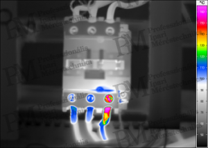
For very precise focusing on small objects, as described at the beginning of the article, do not rely on emitted thermal radiation. If in the visible radiation world, there is sharp contrast in reflected light leading to easier focusing, the same should apply to thermal radiation. Therefore, let's take advantage of this opportunity! The example shown in Image 2 demonstrates focusing for a measurement where due to the particularly high optical magnification, the depth of field is minimal, making correct focusing highly critical. Illuminating with a soldering iron and focusing on the resulting reflected thermal radiation easily and quickly solves this problem.

Practical Temperature Limits of Electrical Equipment

The question often arises where to draw the line between when the detected heating should be considered faulty or even dangerous. Deciding on this issue is particularly difficult when thermography surveys are conducted at significantly lower current levels than the maximum load. To avoid this problem, it is advisable to accept that thermographic condition assessments on electrical equipment should only be carried out when at least 50% of the rated load is present. Only very severe faults can be detected at a load of only 30%.

Accepted threshold values and decision rules (at least 75% load): General threshold values compared to environmental temperature Heating 20 K ... 40 K: to be checked Heating 40 K ... 60 K: to be checked urgently Heating >60 K: critical Threshold values for differences between phases Deviation 5 K ... 20 K: to be checked Deviation 20 K ... 40 K: to be checked urgently Deviation >40 K: critical (** between phases) Threshold values depending on insulating material: Rubber-insulated cables: max. 60°C PVC-insulated cables: max. 70°C Silicone-insulated cables: max. 180°C Other threshold values: Electric motors (measured on cooling fins): depending on type and cooling conditions Insulation class "A" max. 60 ... 80°C Insulation class "B" max. 95 ... 105°C Insulation class "F" max. 115 ... 125°C Insulation class "H" max. 140 ... 150°C Plastic covers: depending on material: max. 50 ... 75°C Magnetic switches: typically max. 85°C Transformers: typically max. 85°C Inside electrical cabinets (IEC/EN 60947-3): max. 35°C Busbars (DIN 43671): max. 65°C External metallic contacts (IEC/EN 60947-3): 80 K (compared to environment) Insulated contacts (IEC/EN 60947-3): 70 K (compared to environment) Note: Lower limits apply for all the above values at lower loads.

Estimation of expected heating under rated load

Heating occurs due to the transient resistance of the examined electrical device (cable, rail, etc.), resulting in energy loss in the form of heat. The device then dissipates this power through radiant heat, convection (towards the air), and heat conduction towards connected elements. The expected heating under higher load (whether current or voltage) is primarily influenced by the load- and temperature-dependent resistance change of the device (or contact). However, the concurrently increasing - expected - heat conduction, radiant heat, and convective heat dissipation also affect the process. Accordingly, determining the resulting heating would require very complex mathematical relationships. In a steady state, in a rail or conductor assumed to be infinitely long, the expected temperature depends on the object and environmental temperature, voltage, current, and many material properties. The latter include the current crowding factor (temperature-dependent), material-specific resistance (temperature-dependent), radiation-based heat transfer coefficient, convective heat transfer coefficient, and the cross-section of the conductor or rail. The equation encompassing all this is quite complex for practical application - especially due to the difficult-to-access material properties - so we recommend using the following estimation instead. Simplified heating estimation under rated load Assuming that the temperature increase between the measurement load and rated load is so small that the temperature change (increase) of the material-specific resistance can be neglected, and neither the current crowding factor nor the heat transfer coefficients change significantly due to the observed device temperature increase, then all these factors can be considered constant in the previous equation. (This can be applied in case of a temperature increase of a few tens of degrees Celsius. However, these simplifications are not valid for larger changes, so the equations below cannot be applied.) Applying the above simplifications, we get the following equation:

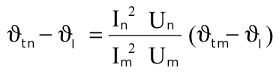
Where: θtn ... estimated object temperature under rated load θtm ... object temperature at the time of thermographic measurement θl ... environmental air temperature (assumed constant) Um ... voltage at the time of thermographic measurement Im ... current at the time of thermographic measurement Un ... rated voltage In ... rated current For network equipment (at constant voltage level), we can use the following equations to estimate the expected absolute temperatures:

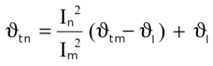
These estimated temperatures can then be compared with the threshold values listed on the previous page.

Examples of electrical equipment faults detectable with thermography

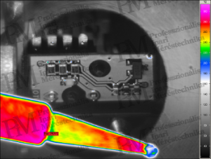
In the article, we aim to demonstrate with the thermal images some typical faults detectable with thermography. The loose screw connection in the thermal images is very instructive in that the strong heating of the washers is clearly visible. The reason for this is that the highest – increased – transient resistance is on both sides of the washers (hence the highest voltage drop and resulting heating), and the incomplete connection of the washers to the nuts results in only a slight dissipation of the heat generated on the washers towards the rest of the structure. In the previous parts of the series, we have tried to provide professional assistance to experts working on low- and medium-voltage electrical equipment for the successful practical application of thermography. In the upcoming parts, we will further complement this with two additional topics: examination procedures aimed at surveying solar cell systems (including solar power plants) and the presentation of the very popular drone-based thermographic applications. Eric Rahne (PIM Ltd.) pim-kft.hu, termokamera.hu

Contact Us

The content of the publication is protected by copyright, and its (even partial) use, electronic or printed re-publication, is only permitted with the indication of the source and author's name, as well as with the author's prior written permission. Infringement of copyright (Copyright) will have legal consequences.